Zero alloc pathfinding in Go
Intro
Algorithms are important. The problem is you can implement the same algorithm so differently.
The implementation performance can range from blazing fast to barely acceptable.
Tutorial: if you see an underlined text that is not a link, hover over it to read a tooltip.
If you like optimizations, specialized data structures and bit tricks then this article is for you.

We’ll concentrate on two algorithms today: A-star and greedy BFS. Both are explained in a brilliant Introduction to the A* Algorithm article.
This article is not about the algorithms themselves, but rather their implementations. I’ll focus on a few tricks that can turn an average A* library into the fastest A* zero alloc library.
Why even bother about the pathfinding, you might ask. I’m doing game development in Go using Ebitengine, and I love it. My Roboden game needed a fast way to build paths: there are many units on the map and they’re independent.
And even though I’ll use Go for every example, the fundamental principles can be used in most other languages.
Evaluating the Existing Libraries
After scanning the awesome-ebitengine and doing some GitHub search, we get these candidates:
- github.com/kelindar/tile
- github.com/beefsack/go-astar
- github.com/fzipp/astar
- github.com/s0rg/grid
- github.com/solarlune/paths
Roboden needs a grid-based pathfinding. Every library from this list can be used for that.
Let’s benchmark them to create a baseline. Every benchmark focuses on a different map kind: from a wall-free map to a maze-like layout.
| Library | Benchmark no_walls (ns) | Benchmark simple_wall (ns) | Benchmark multi_wall (ns) |
|---|---|---|---|
| tile | 107632 ns |
169613 ns |
182342 ns |
| go-astar | 453939 ns |
939300 ns |
1032581 ns |
| astar | 948367 ns |
1554290 ns |
1842812 ns |
| grid | 1816039 ns |
1154117 ns |
1189989 ns |
| paths | 6588751 ns |
5158604 ns |
6114856 ns |
Keep in mind that I discovered the tile library after I made this little research. If we take it out of equotion, you’ll see why I was motivated enough to implement my own library.
Let’s look at the memory allocations for these tests:
| Library | Benchmark no_walls (B/op) | Benchmark simple_wall (B/op) | Benchmark multi_wall (B/op) |
|---|---|---|---|
| tile | 123118 B |
32950 B |
65763 B |
| go-astar | 43653 B |
93122 B |
130731 B |
| astar | 337336 B |
511908 B |
722690 B |
| grid | 996889 B |
551976 B |
740523 B |
| paths | 235168 B |
194768 B |
230416 B |
The last metric is the number of actual allocations:
| Library | Benchmark no_walls | Benchmark simple_wall | Benchmark multi_wall |
|---|---|---|---|
| tile | 3 |
3 |
3 |
| go-astar | 529 |
1347 |
1557 |
| astar | 2008 |
3677 |
3600 |
| grid | 2976 |
1900 |
1759 |
| paths | 7199 |
6368 |
7001 |
The tile library is impressive, but we can still do even better.
Benchmark details for nerds
I’ll start by focusing on the greedy BFS algorithm because I see more optimization opportunities there. The A* will be covered afterwards.
The most performance-sensitive parts of greedy BFS are:
- A tile grid structure
- The result path representation
- A priority queue used for frontier
- An associative array to hold the intermediate results
The Tile Grid
Sometimes I’ll refer to the 2D array elements as cells. Every cell has a coordinate inside a matrix that contains it.
type GridCoord struct {
    X int
    Y int
}
A tile grid maps the world landscape to something meaningful for a pathfinding algorithm. In our case, every cell contains a enum-like value.
type CellType int

// These constants are defined by a user-side.
// You'll see how they're interpreted by the library later.
const (
  CellPlain CellType = iota // 0
  CellSand                  // 1
  CellLava                  // 2
)
Two bits can fit up to four tiles. With this per-cell size, a map of 3600 (60x60) cells will require just 900 bytes.
type Grid struct {
    numCols uint
    numRows uint

    // This slice stores 4 tiles per byte.
    bytes []byte
}
Access to the individual cell will require some extra arithmetics:
func (g *Grid) GetCellTile(c GridCoord) uint8 {
    x := uint(c.X)
    y := uint(c.Y)
    if x >= g.numCols || y >= g.numRows {
        return 0 // Out-of-bounds access
    }
    i := y*g.numCols + x
    byteIndex := i / 4   // MOVL + SHRL
    shift := (i % 4) * 2 // ANDL + SHLL
    return (g.bytes[byteIndex] >> shift) & 0b11
}
Dividing a value by a constant factor (esp. if it’s a power-of-two) can by optimized by the Go compiler quite well. There will be no IDIV instruction in the code above.
Different actors can have different movement types. One actor can only traverse plains, another can also pass through the sand, while airborne units can cross even lava.
This means that a single tile like CellSand can be interpreted differently based on the actor.
Let’s introduce a concept of a layer. A layer maps a tile value stored in the grid from its raw value [0-3] to an actual traversal cost which can exceed this range. Since the max number of tile kinds per grid is 4, only four keys need to be mapped.
type GridLayer [4]byte

// The tile argument value is in [0-3] range.
func (l GridLayer) Get(tile int) byte {
    return l[i]
}
The implicitly inserted bound check can be eliminated:
- return l[i]
+ return l[tile & 0b11]
Layers extend the 2 bits of information to a whole byte. By convention, a value of 0 would mean “blocked” (can’t be traversed). For a greedy BFS any other value would mean a passable cell with a cost of 1. Our A* will treat the non-zero value as an actual traversal cost.
Every movement type will get its own grid layer:
var NormalLayer = pathing.GridLayer{
    CellPlain: 1, // Passable
    CellSand:  0, // Can't traverse
    CellLava:  0, // Can't traverse
}

var FlyingLayer = pathing.GridLayer{
    CellPlain: 1, // Passable
    CellSand:  1, // Passable
    CellLava:  1, // Passable
}
A pathfinding library would use these mapped values instead of the exact tiles themselves. The layer is passed as a BuildPath() function call argument.
My grid map advantages:
- Only 2 bits per cell
- A single grid can be used for different movement types
These 2 bits are not only about saving some memory.
Let’s assume that some machine has a 64-byte wide cache line. The grid map access patterns involve fetching the cell neighbors. The cells to the left and right are always really close. The cells to the up and down will be numCols away from the cell itself. The smaller per-cell size is, the higher the chance that 2*numCols will be located inside the same cache-line.
The Morton order could also be helpful here, but I haven’t tried it.
The Path Object Representation
Almost every library follows a simple path - a path is stored as an array of points.
Let’s take this illustration for example:

The path from {0,1} to {2,3} can look like this:
{0,0} {1,0} {2,0} {2,1} {2,2} {2,3}
But there is another way:
Up Right Right Down Down Down
This kind of encoding requires only 4 values:
type Direction int

const (
    DirRight Direction = iota
    DirDown
    DirLeft
    DirUp
)
You probably already know where I’m going. Four values - two bits.

A single uint64 can fit up to 32 steps. It’s probably not enough, so let’s take a couple of uint64s to make it 64.
To make these packed steps usable, we need a way to iterate over them. I’ll use a couple of bytes for len and pos fields just for that.
const (
    gridPathBytes  = (16 - 2)          // Two bytes are reserved
    gridPathMaxLen = gridPathBytes * 4 // 56
)

type GridPath struct {
    bytes [gridPathBytes]byte
    len   byte
    pos   byte
}
A GridPath object size is 16 bytes. Its memory layout illustrated below.

The individual path elements carry little sense: they can’t be used in isolation. When iterated one by one, hovewer, they encode the entire route. I like to call them deltas because of that.
Just please don’t convert the deltas into an actual slice of points because it ruins the entire idea. Use this path object directly.
GridPath properties:
- The max path length is 56 (it’ll be important later)
- It doesn’t require a heap allocation
- It has a value-semantics, a simple assignment results in deep copy
When a pathfinding algorithm finds a solution, it usually builds a reversed path. Some libraries just return an inversed path while others put an extra effort to inverse the slice elements. If path is iterated in the reverse order, no extra efforts will be required to reverse the actual contents of the path.
The Go compiler starts to place more and more function arguments into registers. A current Go tip in godbolt generates a single MOVUPS instruction to pass the GridPath object (I would rather prefer two MOVQs into a pair of general-purpose registers, but whatever).

The Priority Queue
Only three priority queue operations are needed for our task:
Push(coord, p)- add coordinate to a queuePop() -> (coord, p)- extract a coordinate with a minimal p-valueReset()- clear the queue, keep the memory for re-use
The p priority depends on the exact algorithm. A greedy BFS uses a Manhattan distance between the coord and the finish point.
Based on this description, a minheap sounds like a good fit. We’ll use it for A*. As for the greedy BFS, I found bucket queue to be a better bet.
With each priority value being a separate bucket, the Push operation is straightforward: append to that bucket using p as an index.
The most obvious way to implement a Pop operation is to iterate over the buckets until a non-empty one found. Then element is popped out of this non-empty bucket. Don’t do that.
A max path length of 56 allows us to use a very efficient bitmask approach.
type priorityQueue[T any] struct {
    buckets [64][]T
    mask    uint64
}
With this definition in mind, we’ll start with a Push method.
func (q *priorityQueue[T]) Push(priority int, value T) {
    // A q.buckets[i] boundcheck is removed due to this &-masking.
    i := uint(priority) & 0b111111
    q.buckets[i] = append(q.buckets[i], value)
    q.mask |= 1 << i
}
The q.mask starts with all bits being 0. Whether we push an element into an empty bucket, an associated bit will be set to 1.
The Pop method is more complex, but also very efficient:
func (q *priorityQueue[T]) Pop() T {
    // The TrailingZeros64 on amd64 is a couple of
    // machine instructions (BSF and CMOV).
    //
    // We only need to execute these two to
    // get an index of a non-empty bucket.
    i := uint(bits.TrailingZeros64(q.mask))

    // This explicit length check is needed to remove
    // the q.buckets[i] bound checks below.
    if i < uint(len(q.buckets)) {
        // These two lines perform a pop operation.
        e := q.buckets[i][len(q.buckets[i])-1]
        q.buckets[i] = q.buckets[i][:len(q.buckets[i])-1]

        if len(q.buckets[i]) == 0 {
            // If this bucket is empty now, clear the associated bit.
            // This preserves the invariant.
            q.mask &^= 1 << i
        }
        return e
    }

    // If the queue is empty, return a zero value.
    var x T
    return x
}
To implement a proper Reset, every bucket slice needs to be resliced to zero.
Here is a sad part: all 64 slices will be processed every time, even if most of them are already free. This is where the bitmask shines again.
func (q *priorityQueue[T]) Reset() {
    mask := q.mask

    // The first bucket to clear is the first non-empty one.
    // Skip all empty buckets "to the right".
    offset := uint(bits.TrailingZeros64(mask))
    mask >>= offset
    i := offset

    // When every bucket "to the left" is empty, the mask will be
    // equal to 0 and this loop will terminate.
    for mask != 0 {
        q.buckets[i] = q.buckets[i][:0]
        mask >>= 1
        i++
    }

    q.mask = 0
}
There is a special magic around this implementation. A Reset of an empty queue will reslice exactly 0 buckets. A queue with a single non-empty bucket will require a single bucket reslice. All other cases require a reslicing inside a window. It’s possible to do it a bit differently, but it would require using bits.TrailingZeros64 more than once.
As a bonus that nobody asked for, here is how IsEmpty method can be implemented:
func (q *priorityQueue[T]) IsEmpty() bool {
    return q.mask == 0
}
I would understand if you fell in love with math/bits package after this.

The Best Associative Array
Semantically speaking, we need map[GridCoord]T with only two little differences:
- It should be fast
- It should be easier to re-use its memory
A GridCoord is a struct of two int-typed fields. We can pack the coordinate into a single uint:
func packCoord(numCols int, c GridCoord) uint {
    return uint((c.Y * numCols) + c.X)
}
With a max path length of 56, the search area can be approximated to a square of 56*2+1 cells. Using the search window local coordinates instead of a grid global coordinates makes the packCoord value range quite small: [0-12544].
So instead of thinking in terms of map[GridCoord]T it’s possible to concentrate on map[uint16]T and make our brain take us further.
A first attempt to find a better data structure for this is to use a plain slice. The slice index would be identical to the lookup key. This option has good Get and Set performance, but Reset is slow.
The next step is to consider a sparse map. The Reset becomes very fast at the cost of a slower Get and Set.
My personal recommendation is to use generations map here:
| Data Structure | Set | Get | Reset |
|---|---|---|---|
| slice | 266 |
128 |
6450 |
| generations map | (x1.1) 306 |
(x1.04) 134 |
26 |
| sparse map | (x6.7) 1785 |
(x1.89) 243 |
16 |
| map[uint16]T | (x17.9) 4780 |
(x28.6) 3692 |
1801 |
Going A-star
A couple of changes can turn our greedy BFS into an A*:
- Two generations map instead of one (or one, if elements contain the combined data)
- MinHeap instead of a bucket queue
- A different
pcalculation
The A* can respect the traversal costs without a performance penalty.
How to choose between the greedy bfs and A*?
- By default, you probably want to go with A*
- Greedy BFS works faster and uses less memory
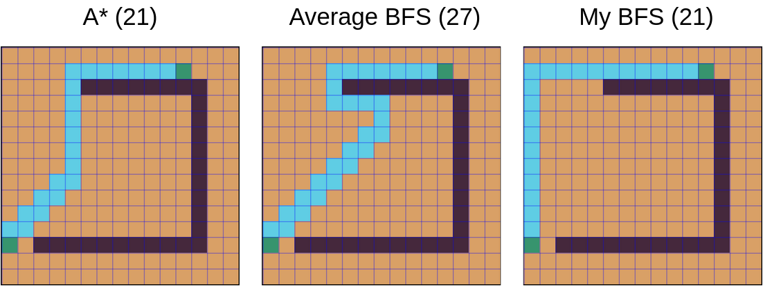
Greedy BFS often managed to find an optimal path, although some complicated maps can confuse it.
When greedy BFS finds an optimal route, it’s almost always a bit different from the route A* would produce. This can be used to produce less predictable paths from your game units. For instance, every odd path can be generated using greedy BFS algorithm and every even path can utilize A*.
Depending on the exact greedy BFS implementation, its quality can be varying. My greedy BFS implementation shows somewhat inspiring results: among many tests, it fails to find an optimal route only a couple of times.
There is also a jump point search, but I didn’t had enough time to take it into account. I may incorporate its ideas into my A* implementation.
The Final Benchmark Results
My new pathing combines everything I described above.
| Library | Benchmark no_walls | Benchmark simple_wall | Benchmark multi_wall |
|---|---|---|---|
| pathing | 3525 ns |
6353 ns |
16927 ns |
| pathing A* | 20140 ns |
35846 ns |
44756 ns |
| tile | 107632 ns |
169613 ns |
182342 ns |
| go-astar | 453939 ns |
939300 ns |
1032581 ns |
| astar | 948367 ns |
1554290 ns |
1842812 ns |
| grid | 1816039 ns |
1154117 ns |
1189989 ns |
| paths | 6588751 ns |
5158604 ns |
6114856 ns |
A* works slower, but it’s still the fastest.
Allocations-wise:
| Library | Benchmark no_walls | Benchmark simple_wall | Benchmark multi_wall |
|---|---|---|---|
| pathing | 0 |
0 |
0 |
| pathing A* | 0 |
0 |
0 |
| tile | 3 |
3 |
3 |
| go-astar | 529 |
1347 |
1557 |
| astar | 2008 |
3677 |
3600 |
| grid | 2976 |
1900 |
1759 |
| paths | 7199 |
6368 |
7001 |

Every single data structure I used supports an efficient memory re-use. A single BuildPath call doesn’t allocate anything. Even the returned path object doesn’t involve the memory allocator.
Is it possible to go even faster? I think so. But for now, I’m quite satisfied with the results.
The promised kelindar/tile library review (optional reading)
Closing Words
The algorithms are important, but their implementations may be paramount. A series of small optimization can have a phenomenal impact.
My library has two major limitations:
- There is a max path length limit - 56
- A single Grid can contain up to 4 tiles (2 bits per cell)
But there are workarounds:
- Partial path-building results can be combined
- Using separate enums per every biome can remove the issue
I could go on, telling that you can increase the limit by using a 32-byte path objects, but you got the idea. Some limitations can enable significant optimizations.
Do you find this article useful for you? If you want to thank me, consider playing my Roboden game. It’s free, multi-platform, open source, and it’s written in Go! I’ll be extra happy if you would write a review. 😇
Useful resources:
- Pathing library source code: github.com/quasilyte/pathing
- Sparse map explained by Russ Cox
- Generations map explained by me
- Roboden game source code: github.com/quasilyte/roboden-game
- Factorio pathfinding blog post
- Ebitengine - a cool game engine for Go
- Awesome Ebitengine list
- I also game a talk on this topic, you can find the slides on speakerdeck